Home > Process Modeling and Simulation Concepts > Functions > Distribution Function

Distribution Function

A function’s intervals always define the percentage of time that a value is returned. For example, if you divide a function into five equal intervals, each corresponding interval value has an equal (20%) chance of being returned by the function.

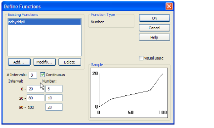
The actual value returned by a distribution function depends on whether the function is continuous or noncontinuous. For example, the following figure illustrates a continuous distribution function.

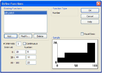
This function has three defined intervals. The intervals specify that 20% of the time the function returns a value between zero and five, 60% of the time it returns a value between five and ten, and 20% of the time it returns a value between 10 and 20. By contrast, the following figure shows the same functions as a noncontinuous function.

In this case, the intervals specify that 20% of the time the function returns a value of five, 60% of the time returns a value of ten, and 20% of the time returns a of 20.

Most iGrafx non-trivial distributions are calculated by ranlib. The actual formula used is

min+(max-min)*genbet(A,B)

Related Topics

See Also